What is Unsupervised Learning and Dimension Reduction | Realcode4you

realcode4you
13 minutes ago
6 min read

What is it and why is it important?

Unsupervised learning is a field in machine learning that deals with data with no pre-existing labels.
Easier to obtain unlabelled data than labelled data, which can require human intervention.
In unsupervised learning , we observe only the p features X_1,X_2, …,X_p involved and goal here is to discover information.
Unsupervised learning is more subjective than supervised learning.
Predictions are not involved, though unsupervised learning can be used as a prequel to supervised learning.

What is it and why is it important?

Techniques for unsupervised learning important in many fields:

Marketing – characterising shoppers based on their behaviour and demographics
Cancers patients – grouped by their gene expressions.

In unsupervised learning, we seek to :

Find an informative way to visualise multivariate data, and
Discover subgroups among the variables/observations.

Multivariate Statistics

What is multivariate statistics?

-Univariate statistics refer to the analysis of a single feature or variable pertaining to the population of interest.

-Multivariate statistics involve the simultaneous observation and analysis of more than one variable.

-Visualising two variables is achieved via scatter plots.

-Visualising three or more variables simultaneously is more complicated.

We can visualise at most in 3-dimensions.
Bivariate and 3-D scatter plots are useful, but do not necessarily reveal the full multivariate relationships.

Linear Combination

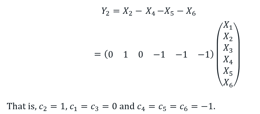
A linear combination is a of creating a new variables by combining several variables through simple addition and/or subtractions of said variables, each of which is multiplied by a coefficient or a scalar value.
Suppose Y is a linear combination of set of p variables, then it can be expressed as:

The selection of c_i is not arbitrary and very much depends on the application of interest.
In many multivariate approaches, c_i’s are also estimated, e.g. principal component analysis.
A linear combination allows us to address questions about certain combinations of variables collectively, instead of individually.
Interpretation of the combination will be important.

Example:

Suppose we have the WA monthly employment data for the past year. The observed variables of interest are:

X_1= number of jobs created;

X_2= number of people hired;

X_3= number of people entered the workforce;

X_4= number of people retired;

X_5= number of people resigned;

X_6= number of people dismissed;

Let Y_1 denote the net employment decrease (NED) in WA this past year. NED can be defined as the total number of jobs lost (retired, resigned or dismissed) minus number of jobs created.

-Let Y_2 denote the net employment increase (NEI) in WA this past year. NEI can be defined as the number of people hired minus the total number of jobs lost (retired, resigned or dismissed).

Principal Component Analysis (PCA)

A multivariate technique that uses orthogonal transformation to convert a set of possibly linearly correlated variables into a set of non-linearly correlated variables, called principal components (PCs).
These PCs are defined as linear combinations of the original set of variables.
PCA is an unsupervised learning technique primarily used as an exploratory tool by ways of dimension reduction.
It often serves as an intermediate step towards other analysis.

The Procedure

A Graphical Illustration:

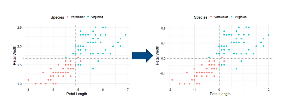
Let’s start with the iris dataset with two variables (features), petal length and petal width, and just between two (see below) of the three species.

A Graphical Illustration:

Step 1: Centre the data, i.e. subtract each x by the mean x ̅.

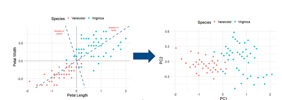
Step 2: Determine the principal components, which formed the new axes.

Step 3: Rotate the new axes so that PC1 is the horizontal axis and PC2 is the vertical axis.

The Procedure (cont’d)

Interpretation

To interpret each component, we must compute the correlation between the original variables and each of the principal components.
Interpretation is then based upon which variable(s) correlate most with each component.
Correlations r that are deemed significant is somewhat subjective.
A threshold is typically selected at r≥0.3, but it also depends on the circumstance.
The components are not always interpretable.

The table below outlines the correlation between each variable and the PCs.

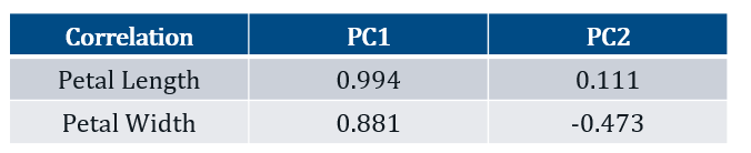
Both variables are strongly, positively, and somewhat equally correlated with PC1. Given that PC1 involves the sum of both variables, one can view the component as a measure of the overall size of the petal.
Petal Length is weakly and positively correlated with PC2, however, Petal Width is moderately and negatively correlated with PC2. One can view this component, PC2, as a measure of petal width. However, given that λ_2=0.056 (i.e. explains ~5% of the variability in the data), it is therefore not of any importance.

Important Notes:

In the iris example, the PCA was based on the raw data.
If the raw data are used, then PCA tend to give more emphasis, i.e. greater loadings, to variables that have greater variability than those with lower variability.
If we wish to give equal weight to each variable, then one should standardised the variables first.
Although standardisation of the variables is typically recommended, the PCA functions in R do not do this by default.

Scree plot

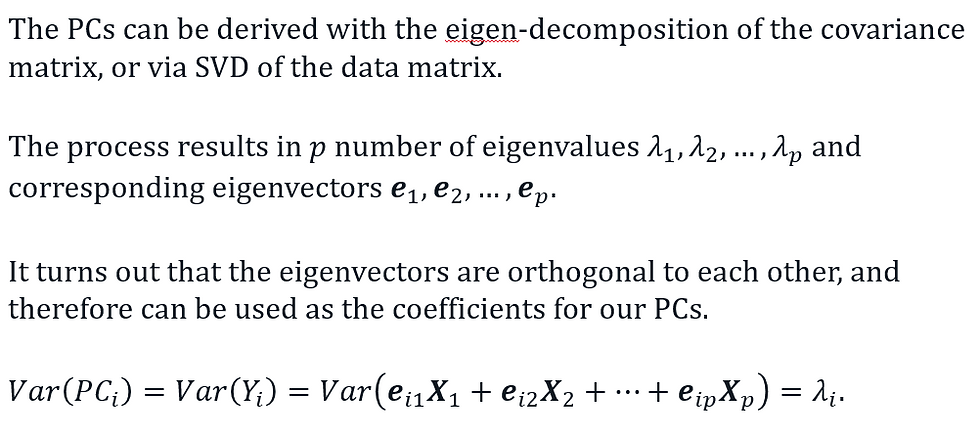
As previously mentioned, when there are p variables involved, there will be p number of PCs to contend with.
However, it often not necessary to examine all PCs and but rather select the first few components that collectively will account for the majority of the variability.
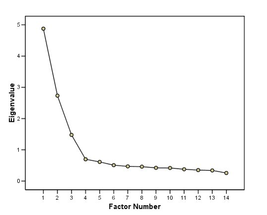
Another way to assess how many components are necessary is by using a scree plot, which is just a line graph of the ordered eigenvalues.

Here, we look for a sharp drop, or alternatively where the plot starts to flatten out.
The scree plot on the right indicates that 3 factors should suffice.
In other words, we have reduced the dimensions from 14 to 3.

Example – Iris dataset with all 4 features

Biplot

A biplot is a exploratory graph that includes information from both samples/individuals (presented a scatter dots) and the variables (presented as vector).
For the variables, the direction and length of the corresponding vectors are dictated by their loadings on the PCs.
Biplots are useful when the individual samples are of interest.
Biplots can be confusing and often time unreadable when there are large numbers of samples and/or variables.

Biplot - How to interpret and what to look for?

PCA plot – Look for clustering or grouping.

Loading plot (vectors)

The length of the vector indicates the importance of the variable.
When two vectors are close and forming a small angle, the two variables they represent are positively correlated.
If two vectors meet each other at 90°, then the variables they represent are uncorrelated.
If two vectors diverge from each other and form an angle close to 180°, then the variables they represent are negatively correlated

PCA plot + loading plot

Focus on the direction of the vectors.
Samples/individuals on the same side of the vector tend to have higher values.
Samples/individuals on the opposite side of the vector tend to have low values.

Biplot – Iris dataset with all 4 features

What can you deduce from the biplot on the right?

Closeness Measures

In order to generate cluster structures from complex multivariate datasets, it is necessary to define “proximity”, “closeness” or “similarity” among the set of objects (samples or variables).
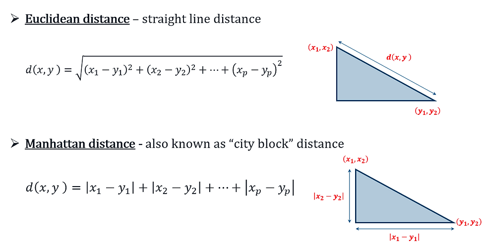
Closeness of samples or individuals is typically defined by some measure of distance such as Euclidean and Manhattan distances, or similarity such as Bray-Curtis Index.
Similarity among variables are grouped on the basis of the aforementioned distance/similarity measures.
Definition of closeness needs to also take into consideration the nature (discrete, continuous, binary) of the variable and the subject matter.

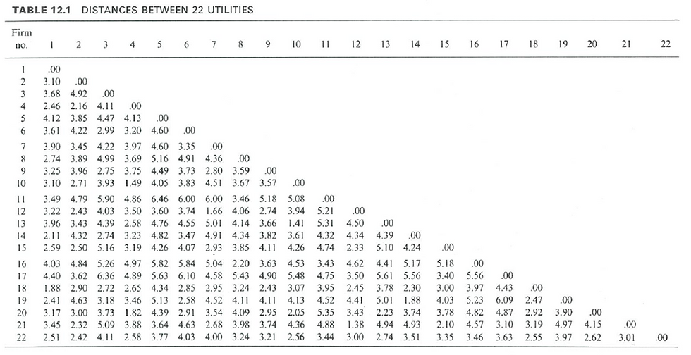
Public utility data of 22 U.S. companies (taken from Johnson and Wichern, 1992)

Euclidean distance matrix on the standardised data

Closeness Measures

Although Euclidean and Manhattan distances can be used for count or binary data, it may not be appropriate to do so.
Consider the data below with p=5 binary variables where 0 = absence and 1 = presence.

Variable 1 is present in both samples, i.e., their distance is 0. Similarly, Variable 3 is absent in both samples and hence, the distance is also 0.
In other words, both 1-1 and 0-0 matches are weighted equally in the context of similarity according to Euclidean/Manhattan distance.

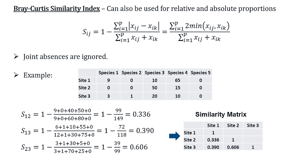
Similarity Measures – Count Data

Similarity Measures – Binary Data

When it comes to binary data, the matches (and mis-matches) for samples i and j may be represented in the form of a contingency table.

There are a number of options available for binary data.

Principal Coordinate Analysis (PCoA)

PCA aims to describe the relationship between the samples based a set of their features.
PCoA (or classical/metric multidimensional scaling) is primarily concern with similarity (based on some measure of distance/similarity) among the samples.
PCoA is equivalent to PCA (vice versa) if Euclidean distance is used.
Euclidean distance does not necessary work well for non-continuous data, and/or when there is a significant amount of zeros.
PCoA allows one to work with other distance/similarity measures.
PCoA works similarly to PCA, but takes in a distance matrix, instead of a covariance or correlation matrix.
It then transform the distance matrix to a set of coordinates such that their Euclidean distances approximates the original distances as well as possible.
Once the mapping in done, it then performs PCA on the constructed coordinates.
The goal of PCoA is preserve the original distances as well possible at lower dimensions.