General Linear Models In Machine Learning | Realcode4you

Terminology for statistical models

Simple

‘Simple’ in simple linear regression refers to the mathematically simplest form of a relationship between two variables which is a straight line y=a+bx.

Linear

Linear in this context means a ‘linear combination’ of variables, it does not mean a straight line. In fact, adding a quadratic term into a statistical regression model is still considered a linear model.

ANOVA

• Usually refers to the variations we saw last week (with any number of factors).

• If it includes a continuous explanatory variable (covariate) it might be called ANCOVA (analysis of covariance).

Regression

Regressus in Latin means ‘to return’. The statistical meaning of the modern word regression is to return one variable to a form of another: to regress y on x (to return y to a form of x).

• The first person to use it statistically didn’t really use it this way, but it ended up catching on for part of his analysis, so now that’s what we call it.

General linear model

• The general form of any linear model for any combination of factors and covariates is a general linear model.

• However, you may find that it can also be called a linear model or simply a regression model.

• The specific words which are used are likely to depend on which discipline or subject area you are in.

• Occasionally a research paper may state that it is using a ‘regression model’ in the abstract, but once you read the methods and results you realise they are actually doing something quite complicated.

Simple linear regression [revision]

x is the independent variable 

y is the dependent variable

(The ‘hat’ on the y means we are referring to the predicted value.)

Finding the line of best fit visually

How good is the model?

Example

Interpreting the intercept and slope

• The null hypothesis for each test is that the parameter = 0

• (Almost) always include an intercept even if it isn’t significant

• Excluding the intercept can force the slope to do something weird

Interpreting the model

• R²: Coefficient of determination

• R² in simple linear regression is the same as r² (correlation squared)

• This is the proportion of variation in the outcome that we can explain with our model.

• In more complicated models the R² is calculated a little differently but interpreted the same way.

• Adjusted R² makes an adjustment based on sample size compared with the number of variables, this is to prevent ‘overfitting’.

What is overfitting?

Fitting too close to the sample data, such that it is unlikely to generalise to the population.

Assumptions of a linear model

1. Suitability & lack of influential outliers: All responses were generated from the same process, so that the same linear model is appropriate for all the observations.

2. Linearity: The linear predictor captures the true relationship between expected value of the response variable and the explanatory variables (and all important explanatory variables are included).

3. Constant variance: The residuals have constant variance.

4. Distribution: The residuals are normally distributed around the predicted values.

5. Independence: The observations are statistically independent of each other.

Four famous datasets – same statistics:

Including more variables in the models

• Interpretation of each variable is similar to anova (factors) and regression (covariates).

• The null hypothesis for each variable is that the difference/slope is zero after adjusting for other variables in the model.

  • If you change the model the p-values will change.

  • Model building & selection we will see next week

• Some additional checks are needed for larger models

Additional checks before analysis

• Are each of the independent variables providing different information?

  • Explore the relationships between the independent variables

  • Scatterplot matrix is helpful

• Residuals versus each of the predictor variables

Examples

1.Exploration

• This will depend on the data and variable types

2.Model statistics

3.Assumptions & residual checks

4.Modifying the model

Example 1 (Body fat and BMI)

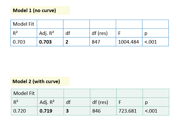
Modifying the model

• There is an extremely slight curve in the data.

• We can try adding this into the model and comparing the model fit and significance.

• The simplest curve to include is a quadratic (squared term).

  • To do this we create a new variable (BMI_squared) and include this as a term in the model.

Example 2 (Elderly and loneliness)

These are the variables we will use from the data. The name of the variable is given in brackets.

You can relabel your variable names if you find that easier if you are following along with the example.

Outcome:

• loneliness (ULSscore)

Covariates:

• depression (PHQ9score)

• anxiety (GAD7score)

• dementia (AD8)

• insomnia (ISI)

With each of these measures a higher score indicates worse symptoms.

Patterns

• ‘Banding’ – data falling into lines

  • Artefact of measuring

  • Not necessarily a problem

• ‘Floor’ effect

  • About 64% of people score the minimum value 6.

  • Many people are not lonely, this feels more like a classification than a continuous measure in this context

  • The measure doesn’t go low enough to capture variation at this end

  • If the measure didn’t go high enough this would be a ‘ceiling’ effect

Modify the model?

• Not really

• Needs a different model

  • Maybe a (zero inflated) Poisson model for count data

  • Maybe classify people as lonely (yes/no) and use logistic regression

  • We will see these later on

For more details you can contact us or send your requirement details at:

realcode4you@gmail.com