Linear Regression with Sea Temperature Trends Using Python Machine Learning

Ocean temperatures are changing fish migratory patterns. Download NOAA’s global average surface temperature anomalies time series data for 1880–2018 from https://www.ncdc.noaa.gov/cag/global/time-series/globe/ocean/1/12/1880-2021 then load and plot the dataset using Seaborn’s regplot function.

What trend do you see?

Implement Linear Regression with this dataset and plot the predicted line together with the dataset.

Implementation

Import Libraries

%matplotlib inline 
import requests 
from io import StringIO
import numpy as np
import pandas as pd
import matplotlib.pyplot as plt
import datetime as dt
import numpy.linalg as lin
from sklearn.svm import SVR
from sklearn.model_selection import GridSearchCV

Import Linear Regression Libraries

#Import scikit learn
from sklearn.linear_model import LinearRegression

Read Data

Linear Regression from the data that looks at all of the gmsl from 1993-2020

#Read data
data = pd.read_csv('/content/sealevel_data__all_1993-2020.csv') # load data set
data.head(2)
data.tail(2)

Output:

Apply LinearRegression Model

X = data.iloc[:, 1].values.reshape(-1, 1)  # values converts it into a numpy array
Y = data.iloc[:, 0].values.reshape(-1, 1)  # -1 means that calculate the dimension of rows, but have 1 column
linear_regressor = LinearRegression()  # create object for the class
linear_regressor.fit(X, Y)  # perform linear regression
Y_pred = linear_regressor.predict(X)  # make predictions

Plot Graph

plt.scatter(X, Y)
plt.plot(X, Y_pred, color='red')
plt.xlabel('Years')
plt.ylabel('Global Mean Sea Level (GMSL) in (mm)')
plt.title('Sea Level over Time 1993-2020(in mm)')
fig1 = plt.gcf()

Output

This visualization shows the model looking at every datapoint taken for the global mass sea level average as it was measured each day.

Linear Regression from the data that takes ONLY the mean of the gmsl from 1993-2015 Grouped by year

X = data_1.iloc[:, 0].values.reshape(-1, 1)  # values converts it into a numpy array
Y = data_1.iloc[:, 1].values.reshape(-1, 1)  # -1 means that calculate the dimension of rows, but have 1 column
linear_regressor = LinearRegression()  # create object for the class
linear_regressor.fit(X, Y)  # perform linear regression
Y_pred = linear_regressor.predict(X)  # make predictions

Plot Graph

#Plot 
plt.scatter(X, Y)
plt.plot(X, Y_pred, color='red')
plt.xlabel('Years')
plt.ylabel('Global Mean Sea Level (GMSL) in (mm)')
plt.title('Sea Level over Time 1993-2015 (in mm)')
fig2 = plt.gcf()

Output:

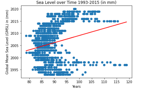
The sea level from 1993 - 2015 showing inconclusive trend over time.

The GMSL is a 1-dimensional time series of globally averaged Sea Surface Height Anomalies (SSHA) from TOPEX/Poseidon, Jason-1, OSTM/Jason-2 and Jason-3. It starts in September 1992 to present, with a lag of up to 4 months. All biases and cross-calibrations have been applied to the data so SSHA are consistent between satellites. Data are reported as changes relative to January 1, 1993 and are 2-month averages. Glacial Isostatic Adjustment (GIA) has been applied. These data are available in ASCII format. Reference: Beckley et al., 2017,

Contact Us or Send your requirement details to get help In any Machine Learning, Data Science Related Help at:

realcode4you@gmail.com