Introduction to Pandas DataFrame | Pandas Dataframe Basics | Realcode4you

Introduction

Pandas is an open source Python library for data analysis. With Panda, the data becomes spreadsheet-like (i.e. with headers and columns) which could be loaded, manipulated, aligned, merged, etc.

Unlike a spreadsheet programme which has its own “macros” language for more complex calculations and analysis, it provides additional features on top of Python, enabling users to automate, reproduce and share analysis across many different operating systems.

Pandas introduces two new data types - Series and DataFrame. The DataFrame represents the entire spreadsheet or rectangle data, whereas the Series is a single column of the DataFrame. A Pandas DataFrame can also be thought of as a dictionary or collection of Series objects.

By using Pandas DataFrame, you can put labels to your variables, making it easier to manage and manipulate data.

Loading Dataset

The first thing we do is to import the Pandas library, then load the data. Afterwards, we can start examining the data.

For the purpose of this Study Unit, we use the data set as sample data from Gapminder (https://www.gapminder.org/) - an independent Swedish foundation that aims to produce fact-based reliable statistics for educational purposes.

You can download the TSV (tab-separated value) files from:

https://github.com/jennybc/gapminder/blob/master/data-raw/04_gap-merged.tsv

and save the file in the same directory where you are running the Python program. Note that when working with Pandas function, it is common practice to give pandas the alias pd when we import the Pandas library.

import pandas as pd
df =pd.read_csv('gapminder.tsv', sep='\t')
print df.head()
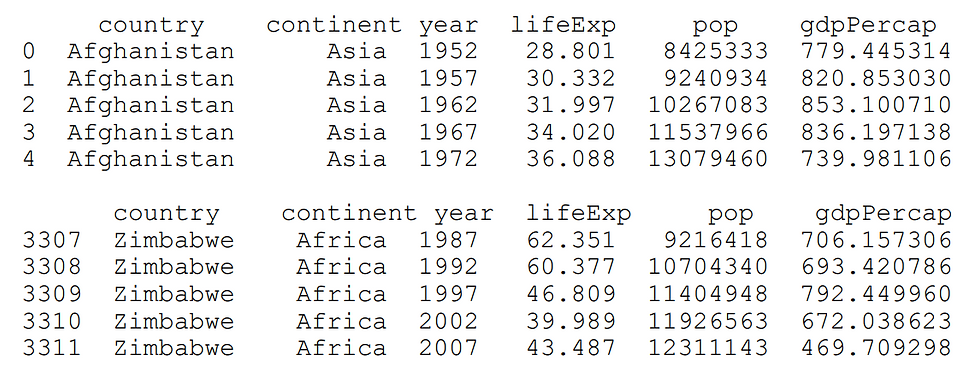
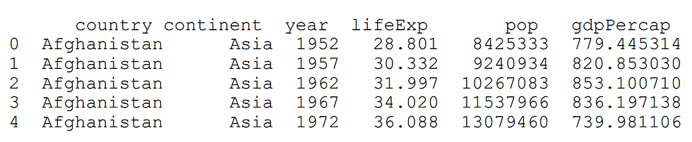
print df.tail()

Note that we have named the sample data file as 'gapminder.tsv'. We import the Pandas library, read the file using the read_csv() method, assuming tabs in the content (i.e. '\t') as separators and then print the first and last five lines of the data.

The code should produce output as follows:

To get the number of rows and columns of the dataframe:

print (df.shape)  
out:  (3312, 6) 

The .shape attribute returns a Python tuple - first value is the number of rows and second the number of columns.

Using the method info() returns more information about the dataset:

print df.info()

out:

RangeIndex: 3312 entries, 0 to 3311
Data columns (total 6 columns):
country 3312 non-null object
continent 3011 non-null object
year 3312 non-null int64
lifeExp 3312 non-null float64
pop 3312 non-null int64
gdpPercap 3312 non-null float64
dtypes: float64(2), int64(2), object(2)
memory usage: 155.3+ KB
None

In the example here, we can see that data in the year column is stored in integer format, whereas lifeExp is stored in float64, which are numbers with decimals. An object type is simply a string, the most common data type.

Selecting Parts of the Dataset

When the information is large, it is difficult to make sense of it when we have to look at all the cells. Hence, there are practical reasons why we want to look at subsets (i.e. parts) of the dataset. There are various ways for us to do so in Pandas DataFrame.

We can select and look at a column, by specifying the name of the column, i.e.

subset_df = df['country'] 

or multiple columns

subset_df = df[['country', 'pop']] 

To select a row, we can specify the row number using the iloc method

print (df.iloc[0]) # returns the first row
print (df.iloc[1]) # returns the second row
print (df.iloc[[1, 3, 5]]) # \
 returns the second, fourth and sixth row
print (df.iloc[-1]) # returns the last row
print (df.iloc[:]) # returns every row

print (df.iloc[:5]  # returns first 5 row row onwards 
print (df.iloc[:5]   # returns first 5 row

Notice that df.iloc[0]returns the first row. The indexing method follows Python style where the first item has the index 0.

The iloc method can also specify column subsets using the indexing method. The syntax is to use square brackets with a comma, like this:

df.iloc[rows, columns] 

Here are some subsetting examples:

df.iloc[:,0] # all rows, first column
df.iloc[:,[2,3]] # all rows, third and fourth column
df.iloc[10:,3:] # 11th rows onwards, fourth column onwards 
df.iloc[10:,:4] # 11th rows onwards, up to fourth column

As you can see, you can use various combination to obtain practically any subset of the data set.

Grouped and Aggregated Calculations

When we work with dataset, it is very common that we want to find answers for sub groups of data, e.g. the average, the count, the total for each grouped set of data.

For example, in our sample data set, we might want to ask questions like:

• For each year, what is the life expectancy average for all countries, or the total population for all countries?

• What if we stratify the data by continent and perform the same calculations?

• Number of countries in each continent?

We answer these questions by performing grouped (i.e. aggregate) calculation. We perform a calculation by applying it to each subset of a variable. We can think of this as a split-apply-combine process. First, the data is split into various parts. A function (or calculation) is applied on each of the split parts. Finally, all the individual split calculation results grouped into a single dataframe.

We do grouped/aggregate computations by using the groupby method on dataframes. To get the answer for average life expectancy by years, we split our data into parts by year, then get the “lifeExp” column and calculate the mean:

year_df = df.groupby('year') 
print(year_df['lifeExp']).mean().head()      # print first 5 rows

output:

year

1950 62.002568

1951 65.904167

1952 49.206867

1953 66.674563

1954 67.459817

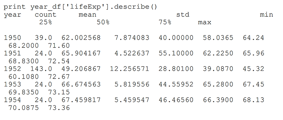
We can also use the method describe() to get a lot more information about the relevant column. You can see that mean() returns the average value:

We can also group and stratify the data by more than one variable. This is done through the use of a list. The following codes group the data by year and continent, then check the mean() of “LifeExpectancy” and “GDPPerCaptia”:

multi_group = df.groupby(['year', 'continent']) 
print(multi_group[['lifeExp','gdpPercap']]).mean() 

Output:

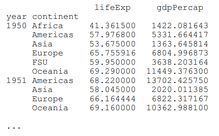
Notice that the data is printed out a little differently. The year and continent column names are not on the same line as the life expectancy and GDP. This is because there is some hierarchical structure between them.

If we need to flatten the dataframe, we use the reset_index method, like this:

flat =  multi_group[['lifeExp','gdpPercap']].mean().reset_index() 
print(flat)

output:

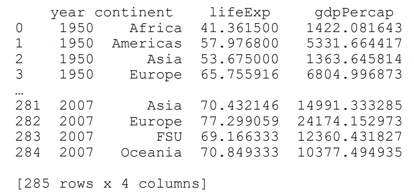
Grouped Frequency Counts

We can also get the frequency statistics of data, by using nunique and value_counts methods respectively, to get counts of unique values and frequency counts.

df.groupby('continent')['country'].nunique()

output:

continent

Africa 51

Americas 25

Asia 41

Europe 35

FSU 6

Oceania 3

Pandas Data Structure

Dataframe Operations

Here, we discuss more ways for you to manipulate the Pandas dataframe, namely, creating, modifying and updating information in the dataframe.

Pandas Series

Pandas Series is a one-dimensional container. You can think of it like a Python list. It is the data type that represents each column of the DataFrame. Note that each column in the dataframe must be of the same data type (dtype).

A simple way to create a Series is to pass in a Python list. If we pass in a list of mixed types, the most common representation of both will be used - typically the object dtype - which is a string/text.

s1 = pd.Series([2, 3, 5])

s2 = pd.Series([2, 'apple'])

print s1

print s2

out:

0 2

1 3

2 5

dtype: int64

0 2

1 apple

dtype: object

Create a DataFrame

We mentioned before that a DataFrame can be thought of as a dictionary of Series object. Hence, using dictionaries are the most common way of creating a DataFrame. The key represents the column name, and the values are the contents of the column.

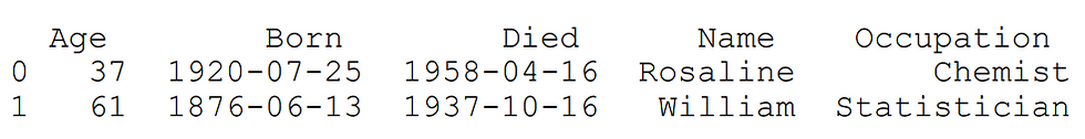
scientists = pd.DataFrame({
 'Name': ['Rosaline','William'],
 'Occupation': ['Chemist', 'Statistician'],
 'Born': ['1920-07-25','1876-06-13'],
 'Died':['1958-04-16','1937-10-16'],
 'Age': [37,61]
 })

print(scientists)

output:

We can use certain parameters to refine the dataframe that we create. For example, we can also use the columns parameter to specify the order of the columns. There is also the index parameter that we can use to specify which column to be set so that the values in this column become the row index.

scientists = pd.DataFrame(
 data = {'Occupation': ['Chemist',\
 'Statistician','Biologists'],
 'Born': ['1920-07-25','1876-06-13','1916-01-23'],
 'Died':['1958-04-16','1937-10-16','1998-01-30'],
 'Age': [37,61,82]},
 index = ['Rosaline','William','John'],
 columns = [ 'Occupation','Age','Born','Died']
 )
print scientists

output:

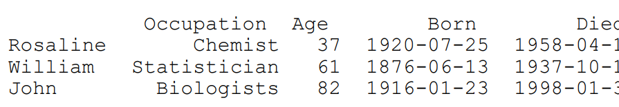
Notice that the first column of the DataFrame is now using name. You can then use the loc[ ] method to specify the row using this syntax:

print scientists.loc['William']
print scientists.loc['William','Age'] # prints 61

which is equivalent to getting the second row of this DataFrame using the iloc[ ] method.

print scientists.iloc[1] 
print scientists.iloc[1,0] 		# prints 'Statistician'

Notice that when we specify a row (or a series of rows), each row is actually a dictionary like object (called Series object in Pandas). You can use its attributes to obtain information about its properties:

row = scientists.loc['William']
print row.keys()
print row.keys()[0] # print the first key
print row.values

Out:

Index([u'Occupation', u'Age', u'Born', u'Died'],

dtype='object')

Occupation

['Statistician' 61 '1876-06-13' '1937-10-16']

Series as a Vector; Boolean Subsetting

In Pandas, when we select a particular column, it returns a Series object where we can operate on it using many methods and functions. A Series is also referred to as a “vector”.

For example, we can select the “Age” column from our scientists dataframe above.

ages = scientists['Age']

This returns a column or series/vector of numbers. From here we can perform various calculations on the entire series/vector:

print ages.mean()
print ages.min()
print ages.max()
print ages.std()
print ages.describe()      # Calculate a summary of statistics

Assume we have a larger dataset that gives us the following results:

ages = scientists['Age']
print ages

out:

0 37

1 61

2 90

3 66

4 56

5 45

6 41

7 41

As before, we can use various vector methods to check its properties, e.g. print

ages.mean()

out:

54.625

We can also set criteria to get back rows that meet those criteria:

print age[age==41] 

Out:

6 41

7 41

Name: age, dtype: int64

print( age[age < age).mean()] 

Out:

0 37

5 45

6 41

7 41

Name: age, dtype: int64

DataFrame Querying and Filtering

We have seen how to select subsets of a dataframe by specifying a combination of row and column indexes or names, using the iloc[ ] and loc[ ] methods. Pandas dataframe columns can also be queried with a boolean expression. Every frame has the module query() as one of its objects members. Having the ability to select subsets of dataframe based on different filtering criteria is an important skill, as you are likely to call upon to query different sets of data based on business input.

we used the gapminder.tsv which contains various population and GDP information about various countries.

country continent year lifeExp pop gdpPercap

0 Afghanistan Asia 1952 28.801 8425333 779.445314

1 Afghanistan Asia 1957 30.332 9240934 820.853030

2 Afghanistan Asia 1962 31.997 10267083 853.100710

3 Afghanistan Asia 1967 34.020 11537966 836.197138

4 Afghanistan Asia 1972 36.088 13079460 739.981106

.... ....

3307 Zimbabwe Africa 1987 62.351 9216418 706.157306

3308 Zimbabwe Africa 1992 60.377 10704340 693.420786

3309 Zimbabwe Africa 1997 46.809 11404948 792.449960

3310 Zimbabwe Africa 2002 39.989 11926563 672.038623

3311 Zimbabwe Africa 2007 43.487 12311143 469.709298

If we want to extract just the rows containing data from a particular year (say 2000), we could use these codes:

import pandas as pd
df =pd.read_csv('gapminder.tsv', sep='\t')
print df.query('year == 2000')

If we want to get rows from year after 2006, we can write

print df.query('year > 2006')

Another effective method is to use the indexing method. Hence, the above results can be achieved similarly using these codes:

print df[(df.year == 2000)]
print df[(df.year > 2006)]

We can even chain multiple filtering criteria. To select all rows where country is Australia and year is more than 2000:

print df[(df.year > 2000) & (df.country == 'Australia')] 

out:

country continent year lifeExp pop gdpPercap

123 Australia NaN 2001 80.350 19357594 30043.24277

124 Australia NaN 2002 80.370 19546792 30687.75473

125 Australia NaN 2003 80.780 19731984 31634.24243

126 Australia NaN 2004 81.150 19913144 32098.50615

127 Australia NaN 2007 81.235 20434176 34435.36744

To select all rows where year is 2000 or 2007:

print df[(df.year == 2000) | (df.year == 2007)]

Take note that in this particular example, df.pop does not refer to the column ‘pop’ . It points to the built-in Python pop() method, which is to remove an item from a list.

http://pandas.pydata.org/pandas-docs/stable/generated/ pandas.DataFrame.pop.html

This is a good illustration of the importance of choosing variable names properly so that they do not clash with built-in Python method names.

Changing DataFrame

In Pandas DataFrame, we can manipulate the data column-wise, and then set the results in a newly created column.

For example, in the gapminder.tsv dataset, we have population figures and GDP per cap figures. To get the GDP figure for each country in every row, we can simply apply the vector calculation like the following:

df['pop'] * df['gdpPercap'] 

If we want to create a new column (say we name it gdp) to store this information, we simply write:

df['gdp'] = df['pop'] * df['gdpPercap']

We can also perform an operation on a vector using a scalar. A scalar is a numeric value, as opposed to a vector of multiple values. Say we want to scale down the gdp number by a million. We can create another column to represent that, after we have scaled down the gdp column:

df['gdp_in_million'] = df['gdp']/1000000 

In this case, every element in the gdp column will be divided by the same scalar value, 100000, and the result is stored in a new column 'gdp_in_million'.

To remove columns from dataframe, we can either specify the columns we want using the column subsetting techniques, or select columns to be removed using the drop method on the dataframe. You can also use the pop method which returns the column you specify while at the same time removes the column from the dataframe:

import pandas as pd
df =pd.read_csv('gapminder.tsv', sep='\t')
# create a new 'gdp' column by doing calculation
# on two column vector-wise
df['gdp'] = df['pop'] * df['gdpPercap']

# create a new 'gdp_in_million' column by doing calculation
# on one column, applying scalar
df['gdp_in_million'] = df['gdp']/1000000

# we drop the column 'gdp' to we create a new dataframe
# new_df; the column 'gdp' still exist in df
# need to provide the axis=1 argument to drop column-wise
new_df = df.drop('gdp', axis=1)

# result is set as the column 'gdp'
# the original df no longer contains the column 'gdp'
result = df.pop('gdp')

Pandas Plotting

Introduction to Plotting

Presenting data in charts and graphs to enable users to better “visualise” the information is an integral part of data processing. Visualising data allows us to better understand the information, and also to see hidden attributes and patterns that will help in data analysis.

In this blog, we will use matplotlib and seaborn libraries to illustrate the plotting capabilities of Python and Pandas. For practical purpose, we recommend that you use Jupyter Notebook (introduced in Study Unit 1) to visualise all output.

Matplotlib

The matplotlib is Python’s fundamental plotting library. It is quite flexible and contains many features that let you control various aspects of the plot. To use it, we import a subpackage called pyplot. Also, it is common practice that when we import it, we give the imported package an abbreviated name, like this:

import matplotlib.pyplot as plt

Let’s use the gapminder.tsv dataset to create our first plot. In the example codes below, we read in the CSV file, create a subset of the dataframe by choosing the year as 2000. Then we create a simple plot with two axes, one showing life Expectancy and the other GDP per capita.

Note that you need to include %matplotlib inline in your codes in order to ensure that the graphs can be displayed properly in a Jupyter Notebook cell.

import pandas as pd
df =pd.read_csv('gapminder.tsv', sep='\t')
subset = df[(df.year == 2000)]
%matplotlib inline
import matplotlib.pyplot as plt
plt.plot(subset['lifeExp'],subset['gdpPercap'], 'o' )

The result is shown in the screenshot here:

From this basic plot, we can immediately see that there is quite strong correlation between GDP per capita and life expectancy (i.e. the wealthier the country is, its citizens are expected to live longer). The ability to gain insight quickly through visualisation demonstrates its power!

Multiple Plots in One Figure

We shall now learn how to use matplotlib to create multiple plots in one figure. This is a convenient way of showing multiple small plots within the same space, instead of showing many plots one after another.

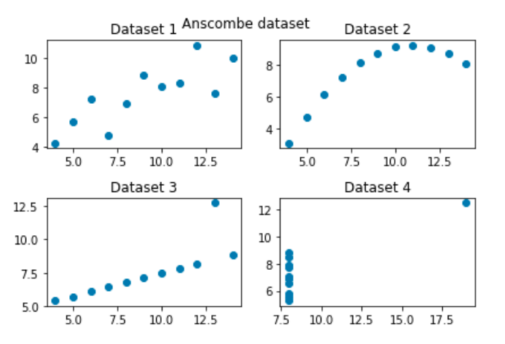
For this purpose, let’s use a data set from seaborn (http://seaborn.pydata.org/) - another Python visualisation library - call Anscombe as sample data. We will be covering more about seaborn in the next Topic.

The Anscombe’s data set contains four sets of data, each of which contains two continuous variables. Each set of data has the same mean, variance, correlation and regression line. However, when we visualise the data, we can see that the information is actually quite distinct for each data set. The purpose of these sample data is to demonstrate the importance of visualisation in data analytics.

To import the data set,

we write:

import seaborn as sns 
anscombe = sns.load_dataset('anscombe') 
print(anscombe) 

output:

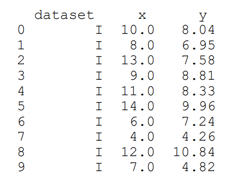
We see that the 4 subsets of the datasets are labelled accordingly. Let’s create subsets of them:

d_1 = anscombe[anscombe['dataset']=='I'] 
d_2 = anscombe[anscombe['dataset']=='II'] 
d_3 = anscombe[anscombe['dataset']=='III'] 
d_4 = anscombe[anscombe['dataset']=='IV'] 

Since there will be four sub plots, we will define the main figure as a 2 x 2 grid. The subplot space is sequentially numbered, with the sub plots placed first in a left to right direction, then from top to bottom.

The following is the complete codes to create the four subplots. You should pay attention to the comments in the codes.

# Need to include this line so that the plots show up in
# Jupyter Notebook
%matplotlib inline
#import the necessary libraries and dataset
import matplotlib.pyplot as plt
import seaborn as sns
anscombe = sns.load_dataset('anscombe')
d_1 = anscombe[anscombe['dataset']=='I']
d_2 = anscombe[anscombe['dataset']=='II']
d_3 = anscombe[anscombe['dataset']=='III']
d_4 = anscombe[anscombe['dataset']=='IV']
# Create the figure where all the subplots will go
fig = plt.figure()

# Define axes1 as the first subplot, which will be the 1st
# plot in the 2 x 2 figure space
axes1 = fig.add_subplot(2,2,1)
# On axes1, we plot the x and y values from dataset d_1
axes1.plot(d_1['x'],d_1['y'], 'o' )
# Set the title for axes1
axes1.set_title('Dataset 1')
# Define axes1 as the first subplot, which will be the 2nd
# plot in the 2 x 2 figure space
axes2 = fig.add_subplot(2,2,2)
# On axes2, we plot the x and y values from dataset d_2
axes2.plot(d_2['x'],d_2['y'], 'o' )
# Set the title for axes2
axes2.set_title('Dataset 2')
# Define axes1 as the first subplot, which will be the 3rd
# plot in the 2 x 2 figure space
axes3 = fig.add_subplot(2,2,3)
# On axes3, we plot the x and y values from dataset d_3
axes3.plot(d_3['x'],d_3['y'], 'o' )
# Set the title for axes3
axes3.set_title('Dataset 3')
# Define axes1 as the first subplot, which will be the 4th
# plot in the 2 x 2 figure space
axes4 = fig.add_subplot(2,2,4)
# On axes4, we plot the x and y values from dataset d_4
axes4.plot(d_4['x'],d_4['y'], 'o' )
# Set the title for axes4
axes4.set_title('Dataset 4')
# Define the title for entire figure
fig.suptitle("Anscombe dataset")
# We use this function to make sure that all the subplots are
 spread out
fig.tight_layout()

If everything goes well, you should be able to see the subplots shown in the screenshot below. Clearly, when the data is visualised, it is very easy to see that even though the data summary statistics are the same, the relationships between the individual data points are very different in each of the data sets.