Implementing Linear Regression and Multiple Linear Regression Using Python Machine Learning
- realcode4you
- Sep 19, 2021
- 2 min read
Linear Regression
Linear regression is perhaps one of the most well known and well understood algorithms in statistics and machine learning.
Importing Related Libraries
import numpy as np
import matplotlib.pyplot as plt
import pandas as pd

%matplotlib inline
First we investigate a simple case by fitting a linear regression for three data points. First we simulate the data:
# simulating the data
x = np.c_[0, 1, 2, 1.5].T
y  = [1, 1.5, 3.1, 1.5]

print(x)
print(y)
Output:
[[0. ] [1. ] [2. ] [1.5]] [1, 1.5, 3.1, 1.5]
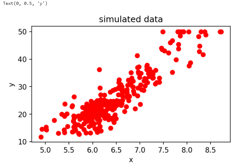
#plotting the data
fig, ax = plt.subplots(figsize=(5, 5), dpi=150)
ax.scatter(x, y, c='r')
ax.set_title('simulated data')
ax.set_xlabel('x')
ax.set_ylabel('y')
Output:

Now we fit the linear regression:
from sklearn import linear_model

# instanciate the model
lr = linear_model.LinearRegression()

# fit the model
lr.fit(x, y)
print("Coefficients:", lr.coef_)
print(" Intercept:", lr.intercept_)
# print " Residues:", lr.residues_output:
Coefficients: [0.89714286] Intercept: 0.7657142857142858
Let's plot the line to see how it estimates our data:
yhat = lr.predict(x)

fig, ax = plt.subplots(figsize=(5, 3), dpi=150)
ax.scatter(x, y, c='r')
ax.plot(x, yhat)

ax.set_title('simulated data and the estimated line')
ax.set_xlabel('x')
ax.set_ylabel('y')
output:

We can use the method predict() to predict y for a new x
x_test = np.c_[4, 2.3].T
y_test = lr.predict(x_test)

print(x_test.T)
print(y_test)
Output:
[[4. 2.3]] [4.35428571 2.82914286]
Multiple Linear Regression
Multiple linear regression attempts to model the relationship between two or more explanatory variables and a response variable by fitting a linear equation to observed data. Every value of the independent variable x is associated with a value of the dependent variable y. For example if we have two explanatory variables (attributes, features), our data has such a form:
Output:

# simulate the data
x = np.c_[[0, 0], [0, 1], [1, 1], [1, 0]].T
y = [1.5, 3.2, 4, 2]

print(x)
print(y)
output:
[[0 0] [0 1] [1 1] [1 0]] [1.5, 3.2, 4, 2]
mlr = linear_model.LinearRegression(fit_intercept=True)
mlr.fit(x,y)
print(mlr.coef_)
print(mlr.intercept_)
Output:
[0.65 1.85] 1.425
print(mlr.predict(x))Output:
[1.425 3.275 3.925 2.075]
Regression for median house prices
We are going to use the package pandas for reading and storing the data.
wget.download('https://github.com/tuliplab/mds/raw/master/Jupyter/data/housing_300.csv')

data = pd.read_csv('housing_300.csv')data.head()output:

data.describe()output:

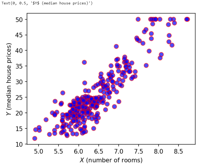
Plot the scatter plot of the number of rooms vs the median house prices.
fig, ax = plt.subplots(figsize=(5, 5), dpi=150)
median_prices = data['MEDV']
avg_rooms = data['RM']
scales = 50*np.ones(len(median_prices))
ax.scatter(avg_rooms, median_prices, color='b',s=scales, alpha=0.7, edgecolor='r')
plt.xlabel('$X$ (number of rooms)')
plt.ylabel('$Y$ (median house prices)')
Output:

print(avg_rooms.shape)
print(median_prices.shape)
Output:
(300,) (300,)
How correlated are the number of rooms and the price of the house?
np.corrcoef(avg_rooms, median_prices)Output:
array([[1. , 0.89804265], [0.89804265, 1. ]])
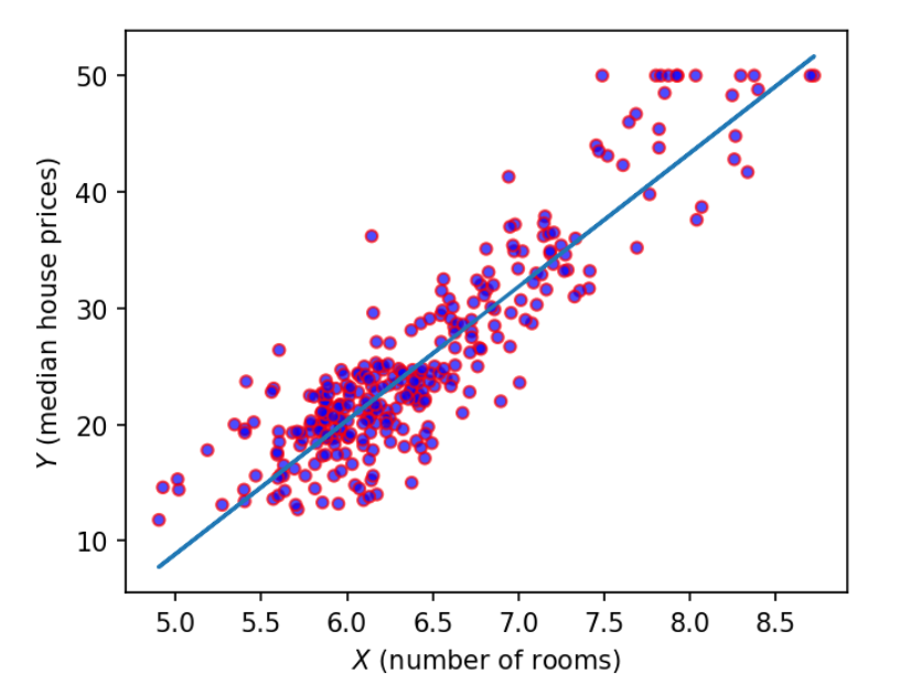
Now we want to fit a linear regression mode on the data.
# prepare the data
x = np.c_[avg_rooms.values]
y = median_prices.tolist()
from sklearn import linear_model
lr = linear_model.LinearRegression()lr.fit(x,y)print(lr.coef_)
print(lr.intercept_)
# print lr.residues_Output:
[11.30440747] -47.09339739688137
# obtain the model parameters
print(lr.coef_, lr.intercept_)
output:
[11.30440747] -47.09339739688137
# predict
yhat = lr.predict(x)
print(x[:10])
print(yhat[:10])
output
[[6.575] [6.421] [7.185] [6.998] [7.147] [6.43 ] [6.012] [6.172] [5.631] [6.004]] [27.23308169 25.49220294 34.12877024 32.01484605 33.69920276 25.59394261 20.86870028 22.67740548 16.56172104 20.77826503]
Output:

Contact Us to get help in Linear Regression machine learning assignment help with an affordable price. Send your request at:


Comments