Image stitching In Machine Learning | Hire Computer Vision Expert
- realcode4you
- May 18, 2022
- 6 min read
1) Image stitching is one of the most successful applications in Computer Vision. Nowadays, it is hard to find a cell phone or an image processing API that does not contain this functionality, In this piece, we will talk about how to perform image stitching using Python and OpenCV. Given a pair of images that share some common region, our goal is to “stitch” them and create a panoramic image scene.
A) An initial and probably naive approach would be to extract key points using an algorithm such as Harris Corners. Then, we could try to match the corresponding key points based on some measure of similarity like Euclidean distance. As we know, corners have one nice property: they are invariant to rotation. It means that, once we detect a corner, if we rotate an image, that corner will still be there. However, what if we rotate then scale an image, causing a problem
In this situation, we would have a hard time because corners are not invariant to scale. That is to say, if we zoom in to an image, the previously detected corner might become a line.
B) Methods like SIFT and SURF try to address the limitations of corner detection algorithms. Usually, corner detector algorithms use a fixed size kernel to detect regions of interest (corners) on images. It is easy to see that when we scale an image, this kernel might become too small or too big. To address this limitation, methods like SIFT use the Difference of Gaussians (DoD). The idea is to apply DoD on differently scaled versions of the same image. It also uses the neighboring pixel information to find and refine key points and corresponding descriptors.
2. By running detectAndCompute() on both, the query and the train image. At this point, we have a set of key points and descriptors for both images. If we use SIFT as the feature extractor, it returns a 128-dimensional feature vector for each key point. If SURF is chosen, we get a 64-dimensional feature vector. The following images show some of the features extracted using SIFT, SURF, BRISK, and ORB.
To make sure the features returned by KNN are well comparable, the authors of the SIFT paper, suggests a technique called ratio test. Basically, we iterate over each of the pairs returned by KNN and perform a distance test. For each pair of features (f1, f2), if the distance between f1 and f2 is within a certain ratio,
we keep it, otherwise, we throw it away. Also, the ratio value must be chosen manually. In essence, ratio testing does the same job as the cross-checking option from the BruteForce Matcher. Both, ensure a pair of detected features are indeed close enough to be considered similar.
3. The bilateral filter smooths an input image while preserving its edges. Each pixel is replaced by a weighted average of its neighbors. Each neighbor is weighted by a spatial component that penalizes distant pixels and a range component that penalizes pixels with a different intensity.
4. Feature detection, description, and matching are essential components of various computer vision applications, thus they have received considerable attention in the last decades. Several feature detectors and descriptors have been proposed in the literature with a variety of definitions for what kind of points in an image is potentially interesting (i.e., a distinctive attribute).
This chapter introduces basic notation and mathematical concepts for detecting and describing image features. Then, it discusses the properties of perfect features and gives an overview of various existing detection and description methods. Furthermore, it explains some approaches to feature matching. Finally, the chapter discusses the most used techniques for performance evaluation of detection and description algorithms
5. A bilateral filter is a non-linear, edge-preserving, and noise-reducing smoothing filter for images. It replaces the intensity of each pixel with a weighted average of intensity values from nearby pixels. This weight can be based on a Gaussian distribution.
Methods such as SIFT and SURF attempt to solve corner algorithms constraints. Corner detector methods often utilize a kernel of defined size to find areas of interest on pictures (corners). It's easy to see that this kernel may go too tiny or too large if you resize a picture.
Methods like SIFT are using Gaussian difference to solve this restriction (DoD). DoD should be applied for copies of the same picture that are different sized. It also uses the next pixel information to locate and improve important spots and descriptions.
We must start by loading 2 pictures, a query picture, and a training picture. Initially, the essential points and descriptors were extracted from both of them. In one stage we may achieve this by utilizing the method OpenCV detect and compute(). Note that we require a keypoint detector instance and the descriptor object to utilize detect and compute(). This may include ORB, SIFT, SURF, etc. In addition, we transform the pictures to grayscale prior to feeding AndCompute().
On both the query and the train picture we execute detect and compute(). We have a number of important points and descriptions for the pictures at this stage. When SIFT is the extractor of the feature, it will return for each key point a 128-dimensional feature vector. When you choose SURF, we obtain a Vector of 64 dimensions. Some features retrieved using SIFT, SURF, BRISK, and ORB are shown in the following photos.
Matching feature
We have many characteristics from both photographs, as we can see. Now we want to compare both attributes and stick to the more like-minded pairings.
OpenCV requires a Matcher object for functional matching. Two tastes are explored here:
Matcher KNN Brute Force (k-Nearest Neighbors)
The Matcher BruteForce (BF) performs what its name says exactly. In view of two sets of characteristics (Figure A & Figure B) individual characteristics of set, A are compared with all characteristics of set B. The Euclidean distance between 2 locations is computed by default. By default.
Implemetation
Import necessary Packages
import cv2
import numpy as np
import matplotlib.pyplot as plt
import imageio
import imutils
cv2.ocl.setUseOpenCL(False)
# select the image id (valid values 1,2,3, or 4)
feature_extractor = 'orb' # one of 'sift', 'surf', 'brisk', 'orb'
feature_matching = 'bf'# read images and transform them to grayscale
# Make sure that the train image is the image that will be transformed
trainImg = imageio.imread('/content/Left.jpg')
trainImg_gray = cv2.cvtColor(trainImg, cv2.COLOR_RGB2GRAY)
queryImg = imageio.imread('/content/Right.jpg')
# Opencv defines the color channel in the order BGR.
# Transform it to RGB to be compatible to matplotlib
queryImg_gray = cv2.cvtColor(queryImg, cv2.COLOR_RGB2GRAY)
fig, (ax1, ax2) = plt.subplots(nrows=1, ncols=2, constrained_layout=False, figsize=(16,9))
ax1.imshow(queryImg, cmap="gray")
ax1.set_xlabel("Query image", fontsize=14)
ax2.imshow(trainImg, cmap="gray")
ax2.set_xlabel("Train image (Image to be transformed)", fontsize=14)
plt.show()
output:

def detectAndDescribe(image, method=None):
    """
    Compute key points and feature descriptors using an specific method
    """

    assert method is not None, "You need to define a feature detection method. Values are: 'sift', 'surf'"

    # detect and extract features from the image
    if method == 'sift':
        descriptor = cv2.xfeatures2d.SIFT_create()
    elif method == 'surf':
        descriptor = cv2.xfeatures2d.SURF_create()
    elif method == 'brisk':
        descriptor = cv2.BRISK_create()
    elif method == 'orb':
        descriptor = cv2.ORB_create()

    # get keypoints and descriptors
    (kps, features) = descriptor.detectAndCompute(image, None)

    return (kps, features)
kpsA, featuresA = detectAndDescribe(trainImg_gray, method=feature_extractor)
kpsB, featuresB = detectAndDescribe(queryImg_gray, method=feature_extractor)
# display the keypoints and features detected on both images
fig, (ax1,ax2) = plt.subplots(nrows=1, ncols=2, figsize=(20,8), constrained_layout=False)
ax1.imshow(cv2.drawKeypoints(trainImg_gray,kpsA,None,color=(0,255,0)))
ax1.set_xlabel("(a)", fontsize=14)
ax2.imshow(cv2.drawKeypoints(queryImg_gray,kpsB,None,color=(0,255,0)))
ax2.set_xlabel("(b)", fontsize=14)
plt.show()Output:

def createMatcher(method,crossCheck):
    "Create and return a Matcher Object"

    if method == 'sift' or method == 'surf':
        bf = cv2.BFMatcher(cv2.NORM_L2, crossCheck=crossCheck)
    elif method == 'orb' or method == 'brisk':
        bf = cv2.BFMatcher(cv2.NORM_HAMMING, crossCheck=crossCheck)
    return bf
def matchKeyPointsBF(featuresA, featuresB, method):
bf = createMatcher(method, crossCheck=True)
# Match descriptors.
best_matches = bf.match(featuresA,featuresB)
# Sort the features in order of distance.
# The points with small distance (more similarity) are ordered first in the vector
rawMatches = sorted(best_matches, key = lambda x:x.distance)
print("Raw matches (Brute force):", len(rawMatches))
return rawMatchesdef matchKeyPointsKNN(featuresA, featuresB, ratio, method):
bf = createMatcher(method, crossCheck=False)
# compute the raw matches and initialize the list of actual matches
rawMatches = bf.knnMatch(featuresA, featuresB, 2)
print("Raw matches (knn):", len(rawMatches))
matches = []
# loop over the raw matches
for m,n in rawMatches:
# ensure the distance is within a certain ratio of each
# other (i.e. Lowe's ratio test)
if m.distance < n.distance * ratio:
matches.append(m)
return matches
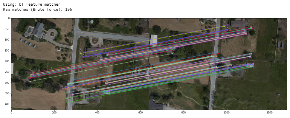
print("Using: {} feature matcher".format(feature_matching))

fig = plt.figure(figsize=(20,8))

if feature_matching == 'bf':
    matches = matchKeyPointsBF(featuresA, featuresB, method=feature_extractor)
    img3 = cv2.drawMatches(trainImg,kpsA,queryImg,kpsB,matches[:100],
                           None,flags=cv2.DrawMatchesFlags_NOT_DRAW_SINGLE_POINTS)
elif feature_matching == 'knn':
    matches = matchKeyPointsKNN(featuresA, featuresB, ratio=0.75, method=feature_extractor)
    img3 = cv2.drawMatches(trainImg,kpsA,queryImg,kpsB,np.random.choice(matches,100),
                           None,flags=cv2.DrawMatchesFlags_NOT_DRAW_SINGLE_POINTS)

plt.imshow(img3)
plt.show()
Output:
def getHomography(kpsA, kpsB, featuresA, featuresB, matches, reprojThresh):
    # convert the keypoints to numpy arrays
    kpsA = np.float32([kp.pt for kp in kpsA])
    kpsB = np.float32([kp.pt for kp in kpsB])

    if len(matches) > 4:

        # construct the two sets of points
        ptsA = np.float32([kpsA[m.queryIdx] for m in matches])
        ptsB = np.float32([kpsB[m.trainIdx] for m in matches])

        # estimate the homography between the sets of points
        (H, status) = cv2.findHomography(ptsA, ptsB, cv2.RANSAC,
            reprojThresh)

        return (matches, H, status)
    else:
        return None
M = getHomography(kpsA, kpsB, featuresA, featuresB, matches, reprojThresh=4)
if M is None:
print("Error!")
(matches, H, status) = M
print(H)Output:
[[ 9.88574951e-01 -1.96849303e-02 3.23358804e+01]
[ 1.61421710e-02 9.80306771e-01 -1.28817626e+02]
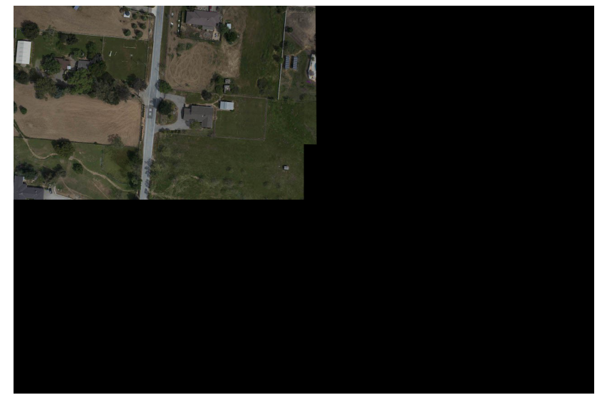
[ 9.46429570e-07 -4.20875802e-05 1.00000000e+00]]# Apply panorama correction
width = trainImg.shape[1] + queryImg.shape[1]
height = trainImg.shape[0] + queryImg.shape[0]
result = cv2.warpPerspective(trainImg, H, (width, height))
result[0:queryImg.shape[0], 0:queryImg.shape[1]] = queryImg
plt.figure(figsize=(20,10))
plt.imshow(result)
plt.axis('off')
plt.show()output
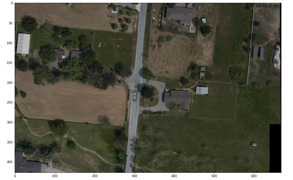
# transform the panorama image to grayscale and threshold it
gray = cv2.cvtColor(result, cv2.COLOR_BGR2GRAY)
thresh = cv2.threshold(gray, 0, 255, cv2.THRESH_BINARY)[1]

# Finds contours from the binary image
cnts = cv2.findContours(thresh.copy(), cv2.RETR_EXTERNAL, cv2.CHAIN_APPROX_SIMPLE)
cnts = imutils.grab_contours(cnts)

# get the maximum contour area
c = max(cnts, key=cv2.contourArea)

# get a bbox from the contour area
(x, y, w, h) = cv2.boundingRect(c)

# crop the image to the bbox coordinates
result = result[y:y + h, x:x + w]

# show the cropped image
plt.figure(figsize=(20,10))
plt.imshow(result)
Output:
To get other help related to OpenCV you can contact Us at:


Comments