Identify Customers to Minimized Loan Delinquency | Data Science Project Help

Context

DRS bank is facing challenging times. Their NPAs (Non-Performing Assets) has been on a rise recently and a large part of these are due to the loans given to individual customers(borrowers). Chief Risk Officer of the bank decides to put in a scientifically robust framework for approval of loans to individual customers to minimize the risk of loans converting into NPAs and initiates a project for the data science team at the bank. You, as a senior member of the team, are assigned this project.

Objective

To identify the criteria to approve loans for an individual customer such that the likelihood of the loan delinquency is minimized

Key questions to be answered

What are the factors that drive the behavior of loan delinquency?

Dataset

• ID: Customer ID

• isDelinquent : indicates whether the customer is delinquent or not (1 => Yes, 0 => No)

• term: Loan term in months

• gender: Gender of the borrower

• age: Age of the borrower

• purpose: Purpose of Loan

• home_ownership: Status of borrower's home

• FICO: FICO (i.e. the bureau score) of the borrower

Domain Information

• Transactor – A person who pays his due amount balance full and on time.

• Revolver – A person who pays the minimum due amount but keeps revolving his balance and does not pay the full amount.

• Delinquent - Delinquency means that you are behind on payments, a person who fails to pay even the minimum due amount.

• Defaulter – Once you are delinquent for a certain period your lender will declare you to be in the default stage.

• Risk Analytics – A wide domain in the financial and banking industry, basically analyzing the risk of the customer.

Import the necessary packages

# this will help in making the Python code more structured automatically (good coding practice)
%load_ext nb_black

# Library to suppress warnings or deprecation notes
import warnings

warnings.filterwarnings("ignore")

# Libraries to help with reading and manipulating data

import pandas as pd
import numpy as np

# Library to split data
from sklearn.model_selection import train_test_split

# libaries to help with data visualization
import matplotlib.pyplot as plt
import seaborn as sns

# Removes the limit for the number of displayed columns
pd.set_option("display.max_columns", None)
# Sets the limit for the number of displayed rows
pd.set_option("display.max_rows", 200)

# Libraries to build decision tree classifier
from sklearn.tree import DecisionTreeClassifier
from sklearn import tree

# To tune different models
from sklearn.model_selection import GridSearchCV

# To perform statistical analysis
import scipy.stats as stats

# To get diferent metric scores
from sklearn.metrics import (
    f1_score,
    accuracy_score,
    recall_score,
    precision_score,
    confusion_matrix,
    plot_confusion_matrix,
    make_scorer,
)

Read the dataset

data = pd.read_csv("Loan_Delinquent_Dataset.csv")
# copying data to another varaible to avoid any changes to original data
loan = data.copy()

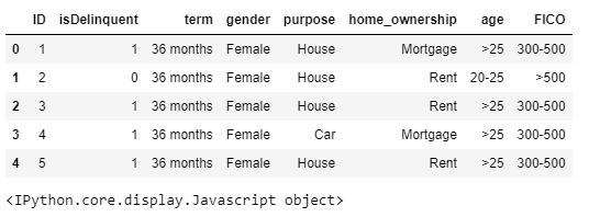
View the first and last 5 rows of the dataset

loan.head()

Output:

Understand the shape of the dataset.

loan.shape

Output:

(11548, 8) <IPython.core.display.Javascript object>

Check the data types of the columns for the dataset

loan.info()

output:

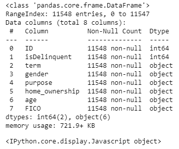
Observations -

• isDelinquent is the dependent variable - type integer.

• All the dependent variables except for ID are object type.

Summary of the dataset.

loan.describe(include="all")

Output:

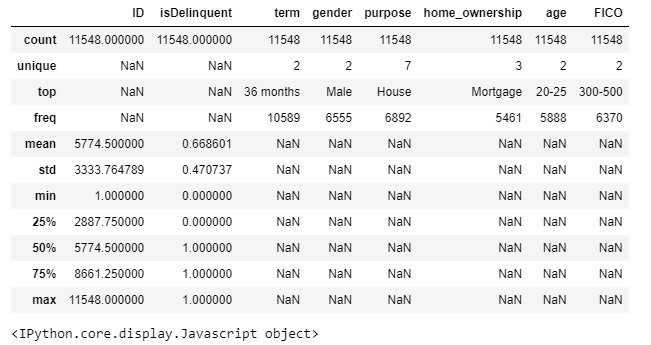
Observations-

• Most of the loans are for a 36-month term loan.

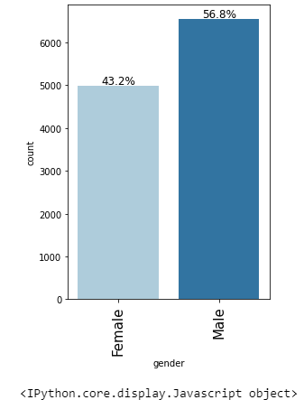
• More males have applied for loans than females.

• Most loan applications are for house loans.

• Most customers have either mortgaged their houses.

• Mostly customers in the age group 20-25 have applied for a loan.

• Most customers have a FICO score between 300 and 500.

# checking for unique values in ID column
loan["ID"].nunique()

output:

11548 <IPython.core.display.Javascript object>

Since all the values in ID column are unique we can drop it

loan.drop(["ID"], axis=1, inplace=True)

Check for missing values

loan.isnull().sum()

output:

Univariate analysis

# function to create labeled barplots
def labeled_barplot(data, feature, perc=False, n=None):
    """
    Barplot with percentage at the top

    data: dataframe
    feature: dataframe column
    perc: whether to display percentages instead of count (default is False)
    n: displays the top n category levels (default is None, i.e., display all levels)
    """

    total = len(data[feature])  # length of the column
    count = data[feature].nunique()
    if n is None:
        plt.figure(figsize=(count + 2, 6))
    else:
        plt.figure(figsize=(n + 2, 6))

    plt.xticks(rotation=90, fontsize=15)
    ax = sns.countplot(
        data=data,
        x=feature,
        palette="Paired",
        order=data[feature].value_counts().index[:n].sort_values(),
    )

    for p in ax.patches:
        if perc == True:
            label = "{:.1f}%".format(
                100 * p.get_height() / total
            )  # percentage of each class of the category
        else:
            label = p.get_height()  # count of each level of the category

        x = p.get_x() + p.get_width() / 2  # width of the plot
        y = p.get_height()  # height of the plot

        ax.annotate(
            label,
            (x, y),
            ha="center",
            va="center",
            size=12,
            xytext=(0, 5),
            textcoords="offset points",
        )  # annotate the percentage

    plt.show()  # show the plot

Observations on isDelinquent

labeled_barplot(loan, "isDelinquent", perc=True)

output:

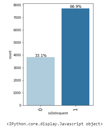
• 66.9% of the customers are delinquent

Observations on term

labeled_barplot(loan, "term", perc=True)

output:

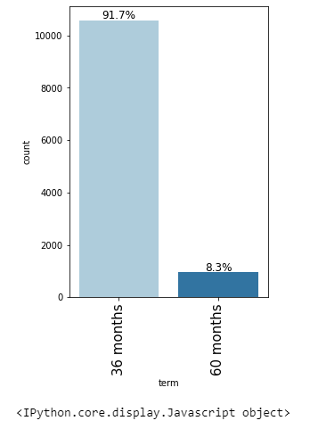
• 91.7% of the loans are for a 36 month term.

Observations on gender

labeled_barplot(loan, "gender", perc=True)

output

Observations on purpose

labeled_barplot(loan, "purpose", perc=True)

output:

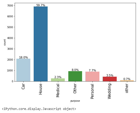
• Most loan applications are for house loans (59.7%) followed by car loans (18%)

• There are 2 levels named 'other' and 'Other' under the purpose variable. Since we do not have any other information about these, we can merge these levels.

Observations on home_ownership

labeled_barplot(loan, "home_ownership", perc=True)

output:

• Very few applicants <10% own their house, Most customers have either mortgaged their houses or live on rent.

Observations on age

labeled_barplot(loan, "age", perc=True)

output:

Data Cleaning

loan["purpose"].unique()

output:

array(['House', 'Car', 'Other', 'Personal', 'Wedding', 'Medical', 'other'], dtype=object) <IPython.core.display.Javascript object>

We can merge the purpose - 'other' and 'Other' together

loan["purpose"].replace("other", "Other", inplace=True)

loan["purpose"].unique()

output:

array(['House', 'Car', 'Other', 'Personal', 'Wedding', 'Medical'], dtype=object) <IPython.core.display.Javascript object>

Bivariate Analysis

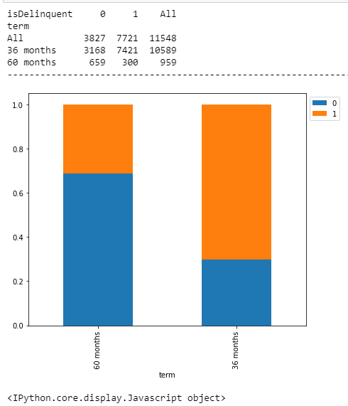
# function to plot stacked bar chart
def stacked_barplot(data, predictor, target):
    """
    Print the category counts and plot a stacked bar chart

    data: dataframe
    predictor: independent variable
    target: target variable
    """
    count = data[predictor].nunique()
    sorter = data[target].value_counts().index[-1]
    tab1 = pd.crosstab(data[predictor], data[target], margins=True).sort_values(
        by=sorter, ascending=False
    )
    print(tab1)
    print("-" * 120)
    tab = pd.crosstab(data[predictor], data[target], normalize="index").sort_values(
        by=sorter, ascending=False
    )
    tab.plot(kind="bar", stacked=True, figsize=(count + 5, 6))
    plt.legend(
        loc="lower left", frameon=False,
    )
    plt.legend(loc="upper left", bbox_to_anchor=(1, 1))
    plt.show()

stacked_barplot(loan, "term", "isDelinquent")

output:

Model Building - Approach

1. Data preparation

2. Partition the data into train and test set.

3. Built a CART model on the train data.

4. Tune the model and prune the tree, if required.

Split Data

X = loan.drop(["isDelinquent"], axis=1)
y = loan["isDelinquent"]

# encoding the categorical variables
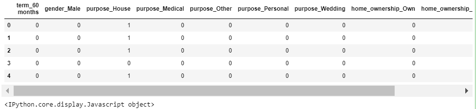
X = pd.get_dummies(X, drop_first=True)
X.head()

output:

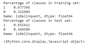
X_train, X_test, y_train, y_test = train_test_split(X, y, test_size=0.4, random_state=1)

print("Number of rows in train data =", X_train.shape[0])
print("Number of rows in test data =", X_test.shape[0])

print("Percentage of classes in training set:")
print(y_train.value_counts(normalize=True))
print("Percentage of classes in test set:")
print(y_test.value_counts(normalize=True))

output:

Build Decision Tree Model Model evaluation criterion Model can make wrong predictions as:

1. Predicting a customer will not be behind on payments (Non-Delinquent) but in reality the customer would be behind on payments.

2. Predicting a customer will be behind on payments (Delinquent) but in reality the customer would not be behind on payments (Non-Delinquent).

Which case is more important?

• If we predict a non-delinquent customer as a delinquent customer bank would lose an opportunity of providing loan to a potential customer.

How to reduce this loss i.e need to reduce False Negatives?

• recall should be maximized, the greater the recall higher the chances of minimizing the false negatives.

First, let's create functions to calculate different metrics and confusion matrix so that we don't have to use the same code repeatedly for each model.

• The model_performance_classification_sklearn function will be used to check the model performance of models.

• The make_confusion_matrix function will be used to plot confusion matrix.

# defining a function to compute different metrics to check performance of a classification model built using sklearn
def model_performance_classification_sklearn(model, predictors, target):
    """
    Function to compute different metrics to check classification model performance

    model: classifier
    predictors: independent variables
    target: dependent variable
    """

    # predicting using the independent variables
    pred = model.predict(predictors)

    acc = accuracy_score(target, pred)  # to compute Accuracy
    recall = recall_score(target, pred)  # to compute Recall
    precision = precision_score(target, pred)  # to compute Precision
    f1 = f1_score(target, pred)  # to compute F1-score

    # creating a dataframe of metrics
    df_perf = pd.DataFrame(
        {"Accuracy": acc, "Recall": recall, "Precision": precision, "F1": f1,},
        index=[0],
    )

    return df_perf

def confusion_matrix_sklearn(model, predictors, target):
    """
    To plot the confusion_matrix with percentages

    model: classifier
    predictors: independent variables
    target: dependent variable
    """
    y_pred = model.predict(predictors)
    cm = confusion_matrix(target, y_pred)
    labels = np.asarray(
        [
            ["{0:0.0f}".format(item) + "\n{0:.2%}".format(item / cm.flatten().sum())]
            for item in cm.flatten()
        ]
    ).reshape(2, 2)

    plt.figure(figsize=(6, 4))
    sns.heatmap(cm, annot=labels, fmt="")
    plt.ylabel("True label")
    plt.xlabel("Predicted label")

Build Decision Tree Model

model = DecisionTreeClassifier(criterion="gini", random_state=1)
model.fit(X_train, y_train)

output:

DecisionTreeClassifier(random_state=1) <IPython.core.display.Javascript object>

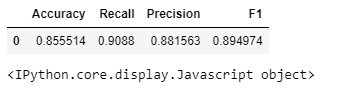
Checking model performance on training set

decision_tree_perf_train = model_performance_classification_sklearn(
    model, X_train, y_train
)
decision_tree_perf_train

output:

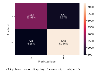
confusion_matrix_sklearn(model, X_train, y_train)

output: