Exploratory data analysis (EDA) In Python Machine Learning
- realcode4you
- Jun 26, 2021
- 4 min read
Basic Terminology
What is EDA?
Data-point/vector/Observation
Data-set.
Feature/Variable/Input-variable/Dependent-varibale
Label/Indepdendent-variable/Output-varible/Class/Class-label/Response label
Vector: 2-D, 3-D, 4-D,.... n-D
Q. What is a 1-D vector: Scalar
Iris Flower dataset
Toy Dataset: Iris Dataset: [https://en.wikipedia.org/wiki/Iris_flower_data_set]
A simple dataset to learn the basics.
3 flowers of Iris species. [see images on wikipedia link above]
1936 by Ronald Fisher.
Petal and Sepal: http://terpconnect.umd.edu/~petersd/666/html/iris_with_labels.jpg
Objective: Classify a new flower as belonging to one of the 3 classes given the 4 features.
Importance of domain knowledge.
Why use petal and sepal dimensions as features?
Why do we not use 'color' as a feature?
Import All Related Libraries
import pandas as pd
import seaborn as sns
import matplotlib.pyplot as plt
import numpy as np
Download Datasets
'''downlaod iris.csv from https://raw.githubusercontent.com/uiuc-cse/data-fa14/gh-pages/data/iris.csv'''
#Load Iris.csv into a pandas dataFrame.
iris = pd.read_csv("iris.csv")
Checking Shape Of dataset
# (Q) how many data-points and features?
print (iris.shape)
Output
(150, 5)
Checking Columns
#(Q) What are the column names in our dataset?
print (iris.columns)
Output
Index(['sepal_length', 'sepal_width', 'petal_length', 'petal_width', 'species'], dtype='object')
Count the flowers of each species
#(or) How many flowers for each species are present?

iris["species"].value_counts()
# balanced-dataset vs imbalanced datasets
#Iris is a balanced dataset as the number of data points for every class is 50.
Output
virginica 50 setosa 50 versicolor 50 Name: species, dtype: int64
2-D Scatter Plot
#2-D scatter plot:
#ALWAYS understand the axis: labels and scale.

iris.plot(kind='scatter', x='sepal_length', y='sepal_width') ;
plt.show()

#cannot make much sense out it.
#What if we color the points by thier class-label/flower-type.
Output

2-D Scatter plot with color-coding for each flower type/class.
# Here 'sns' corresponds to seaborn.
sns.set_style("whitegrid");
sns.FacetGrid(iris, hue="species", size=4) \
   .map(plt.scatter, "sepal_length", "sepal_width") \
   .add_legend();
plt.show();
Output
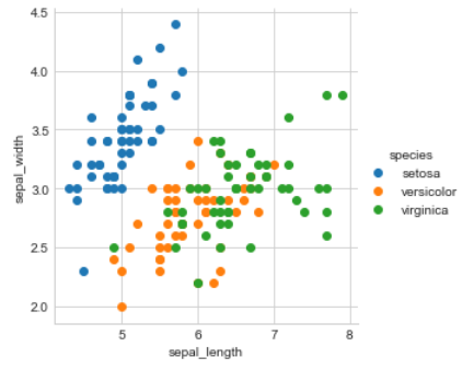
Observation(s):
Using sepal_length and sepal_width features, we can distinguish Setosa flowers from others.
Seperating Versicolor from Viginica is much harder as they have considerable overlap.
3D Scatter plot
Needs a lot to mouse interaction to interpret data.
What about 4-D, 5-D or n-D scatter plot?
Pair-plot
# pairwise scatter plot: Pair-Plot
# Dis-advantages:
##Can be used when number of features are high.
##Cannot visualize higher dimensional patterns in 3-D and 4-D.
#Only possible to view 2D patterns.
plt.close();
sns.set_style("whitegrid");
sns.pairplot(iris, hue="species", size=3);
plt.show()
# NOTE: the diagnol elements are PDFs for each feature. PDFs are expalined below.
output:


Observations
petal_length and petal_width are the most useful features to identify various flower types.
While Setosa can be easily identified (linearly seperable), Virnica and Versicolor have some overlap (almost linearly seperable).
We can find "lines" and "if-else" conditions to build a simple model to classify the flower types.
Histogram, PDF, CDF
# What about 1-D scatter plot using just one feature?
#1-D scatter plot of petal-length
import numpy as np
iris_setosa = iris.loc[iris["species"] == "setosa"];
iris_virginica = iris.loc[iris["species"] == "virginica"];
iris_versicolor = iris.loc[iris["species"] == "versicolor"];

#print(iris_setosa["petal_length"])
plt.plot(iris_setosa["petal_length"], np.zeros_like(iris_setosa['petal_length']), 'o')
plt.plot(iris_versicolor["petal_length"], np.zeros_like(iris_versicolor['petal_length']), 'o')
plt.plot(iris_virginica["petal_length"], np.zeros_like(iris_virginica['petal_length']), 'o')

plt.show()
#Disadvantages of 1-D scatter plot: Very hard to make sense as points
#are overlapping a lot.
#Are there better ways of visualizing 1-D scatter plots?
Output:

Petal Length
sns.FacetGrid(iris, hue="species", size=5) \
   .map(sns.distplot, "petal_length") \
   .add_legend();
plt.show();
Output:

Petal Width
sns.FacetGrid(iris, hue="species", size=5) \
   .map(sns.distplot, "petal_width") \
   .add_legend();
plt.show();
Output:

Sepal Length
sns.FacetGrid(iris, hue="species", size=5) \
   .map(sns.distplot, "sepal_length") \
   .add_legend();
plt.show();
Output

Sepal Width
sns.FacetGrid(iris, hue="species", size=5) \
   .map(sns.distplot, "sepal_width") \
   .add_legend();
plt.show();
Output

CDF Petal Length
#Plot CDF of petal_length

counts, bin_edges = np.histogram(iris_setosa['petal_length'], bins=10,
                                 density = True)
pdf = counts/(sum(counts))
print(pdf);
print(bin_edges);
cdf = np.cumsum(pdf)
plt.plot(bin_edges[1:],pdf);
plt.plot(bin_edges[1:], cdf)
counts, bin_edges = np.histogram(iris_setosa['petal_length'], bins=20,
                                 density = True)
pdf = counts/(sum(counts))
plt.plot(bin_edges[1:],pdf);

plt.show();
Output
[ 0.02 0.02 0.04 0.14 0.24 0.28 0.14 0.08 0. 0.04] [ 1. 1.09 1.18 1.27 1.36 1.45 1.54 1.63 1.72 1.81 1.9 ]

# Need for Cumulative Distribution Function (CDF)
# We can visually see what percentage of versicolor flowers have a
# petal_length of less than 1.6?
# How to construct a CDF?
# How to read a CDF?

#Plot CDF of petal_length

counts, bin_edges = np.histogram(iris_setosa['petal_length'], bins=10,
                                 density = True)
pdf = counts/(sum(counts))
print(pdf);
print(bin_edges)

#compute CDF
cdf = np.cumsum(pdf)
plt.plot(bin_edges[1:],pdf)
plt.plot(bin_edges[1:], cdf)
plt.show();
Output
[ 0.02 0.02 0.04 0.14 0.24 0.28 0.14 0.08 0. 0.04] [ 1. 1.09 1.18 1.27 1.36 1.45 1.54 1.63 1.72 1.81 1.9 ]

Plots of CDF of petal_length for various types of flowers
# Misclassification error if you use petal_length only.

counts, bin_edges = np.histogram(iris_setosa['petal_length'], bins=10,
                                 density = True)
pdf = counts/(sum(counts))
print(pdf);
print(bin_edges)
cdf = np.cumsum(pdf)
plt.plot(bin_edges[1:],pdf)
plt.plot(bin_edges[1:], cdf)


# virginica
counts, bin_edges = np.histogram(iris_virginica['petal_length'], bins=10,
                                 density = True)
pdf = counts/(sum(counts))
print(pdf);
print(bin_edges)
cdf = np.cumsum(pdf)
plt.plot(bin_edges[1:],pdf)
plt.plot(bin_edges[1:], cdf)


#versicolor
counts, bin_edges = np.histogram(iris_versicolor['petal_length'], bins=10,
                                 density = True)
pdf = counts/(sum(counts))
print(pdf);
print(bin_edges)
cdf = np.cumsum(pdf)
plt.plot(bin_edges[1:],pdf)
plt.plot(bin_edges[1:], cdf)

plt.show();
Output
[ 0.02 0.02 0.04 0.14 0.24 0.28 0.14 0.08 0. 0.04] [ 1. 1.09 1.18 1.27 1.36 1.45 1.54 1.63 1.72 1.81 1.9 ] [ 0.02 0.1 0.24 0.08 0.18 0.16 0.1 0.04 0.02 0.06] [ 4.5 4.74 4.98 5.22 5.46 5.7 5.94 6.18 6.42 6.66 6.9 ] [ 0.02 0.04 0.06 0.04 0.16 0.14 0.12 0.2 0.14 0.08] [ 3. 3.21 3.42 3.63 3.84 4.05 4.26 4.47 4.68 4.89 5.1 ]

Mean, Variance and Std-dev
#Mean, Variance, Std-deviation,
print("Means:")
print(np.mean(iris_setosa["petal_length"]))

#Mean with an outlier.
print(np.mean(np.append(iris_setosa["petal_length"],50)));
print(np.mean(iris_virginica["petal_length"]))
print(np.mean(iris_versicolor["petal_length"]))

print("\nStd-dev:");
print(np.std(iris_setosa["petal_length"]))
print(np.std(iris_virginica["petal_length"]))
print(np.std(iris_versicolor["petal_length"]))
Output
Means:
1.464
2.41568627451
5.552
4.26
Std-dev:
0.171767284429
0.546347874527
0.465188133985
Median, Percentile, Quantile, IQR, MAD
#Median, Quantiles, Percentiles, IQR.
print("\nMedians:")
print(np.median(iris_setosa["petal_length"]))

#Median with an outlier
print(np.median(np.append(iris_setosa["petal_length"],50)));
print(np.median(iris_virginica["petal_length"]))
print(np.median(iris_versicolor["petal_length"]))


print("\nQuantiles:")
print(np.percentile(iris_setosa["petal_length"],np.arange(0, 100, 25)))
print(np.percentile(iris_virginica["petal_length"],np.arange(0, 100, 25)))
print(np.percentile(iris_versicolor["petal_length"], np.arange(0, 100, 25)))

print("\n90th Percentiles:")
print(np.percentile(iris_setosa["petal_length"],90))
print(np.percentile(iris_virginica["petal_length"],90))
print(np.percentile(iris_versicolor["petal_length"], 90))

from statsmodels import robust
print ("\nMedian Absolute Deviation")
print(robust.mad(iris_setosa["petal_length"]))
print(robust.mad(iris_virginica["petal_length"]))
print(robust.mad(iris_versicolor["petal_length"]))
Output
Medians: 1.5 1.5 5.55 4.35 Quantiles: [ 1. 1.4 1.5 1.575] [ 4.5 5.1 5.55 5.875] [ 3. 4. 4.35 4.6 ] 90th Percentiles: 1.7 6.31 4.8 Median Absolute Deviation 0.148260221851 0.667170998328 0.518910776477
Box plot and Whiskers
#Box-plot with whiskers: another method of visualizing the  1-D scatter plot more intuitivey.
# The Concept of median, percentile, quantile.
# How to draw the box in the box-plot?
# How to draw whiskers: [no standard way] Could use min and max or use other complex statistical techniques.
# IQR like idea.

#NOTE: IN the plot below, a technique call inter-quartile range is used in plotting the whiskers.
#Whiskers in the plot below donot correposnd to the min and max values.

#Box-plot can be visualized as a PDF on the side-ways.

sns.boxplot(x='species',y='petal_length', data=iris)
plt.show()
Output

Violin plots
# A violin plot combines the benefits of the previous two plots
#and simplifies them

# Denser regions of the data are fatter, and sparser ones thinner
#in a violin plot

sns.violinplot(x="species", y="petal_length", data=iris, size=8)
plt.show()
Output

Contact us to get any other visualization help related to R programming, python machine learning, D3.js or using the tableau at:
realcode4you@gmail.com and get instant help with affordable prices.
We are always focus to delivered unique or without plagiarism code which is written by our highly educated professional which provide well structured code within your given time frame.
If you are looking other programming language help like C, C++, Java, Python, PHP, Asp.Net, NodeJs, ReactJs, etc. with the different types of databases like MySQL, MongoDB, SQL Server, Oracle, etc. then also contact us.


Comments