Agglomerative Hierarchical Clustering Dendogram Assignment Help | What is Hierarchical Clustering?

Import Necessary Packages

import pandas as pd
import numpy as np
import matplotlib.pyplot as plt 
%matplotlib inline
from scipy.stats import zscore
import seaborn as sns

Read Data

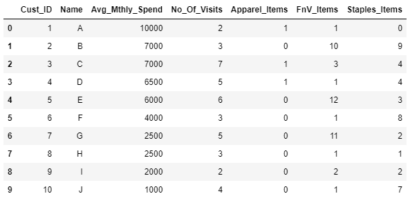
# reading the CSV file into pandas dataframe
custData = pd.read_csv("Cust_Spend_Data.csv") 
custData.head(10)

Output:

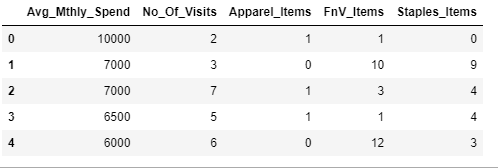
custDataAttr=custData.iloc[:,2:]
custDataAttr.head()

Output:

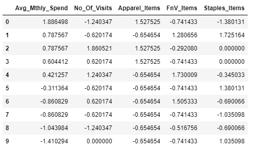
custDataScaled=custDataAttr.apply(zscore)
custDataScaled.head(10)

Output:

#importing seaborn for statistical plots
sns.pairplot(custDataScaled, height=2,aspect=2 , diag_kind='kde')

Output:

from sklearn.cluster import AgglomerativeClustering 
model = AgglomerativeClustering(n_clusters=3, affinity='euclidean',  linkage='average')
model.fit(custDataScaled)

Output:

AgglomerativeClustering(affinity='euclidean', compute_full_tree='auto',
            connectivity=None, linkage='average', memory=None,
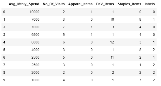
            n_clusters=3, pooling_func='deprecated')

custDataAttr['labels'] = model.labels_
custDataAttr.head(10)
#custDataAttr.groupby(["labels"]).count()

Output:

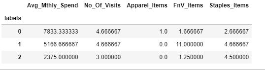
custDataClust = custDataAttr.groupby(['labels'])
custDataClust.mean()

Output:

from scipy.cluster.hierarchy import cophenet, dendrogram, linkage
from scipy.spatial.distance import pdist  #Pairwise distribution between data points

# cophenet index is a measure of the correlation between the distance of points in feature space and distance on dendrogram
# closer it is to 1, the better is the clustering
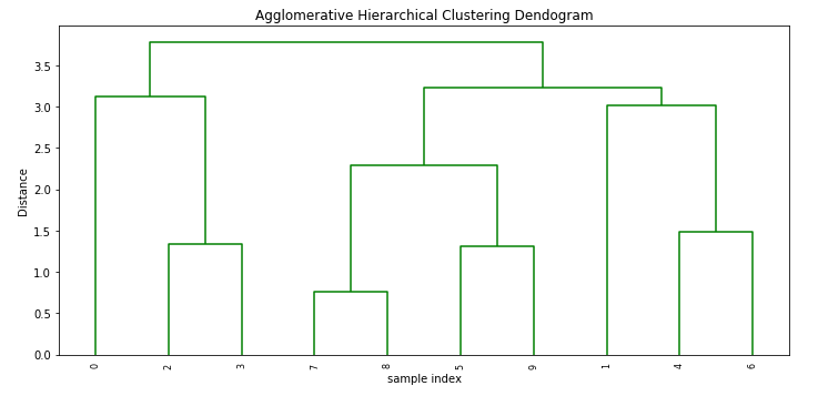
Z = linkage(custDataScaled, metric='euclidean', method='average')
c, coph_dists = cophenet(Z , pdist(custDataScaled))
c

Output:

0.8681149436293064

plt.figure(figsize=(10, 5))
plt.title('Agglomerative Hierarchical Clustering Dendogram')
plt.xlabel('sample index')
plt.ylabel('Distance')
dendrogram(Z, leaf_rotation=90.,color_threshold = 40, leaf_font_size=8. )
plt.tight_layout()

Output:

# cophenet index is a measure of the correlation between the distance of points in feature space and distance on dendrogram
# closer it is to 1, the better is the clustering

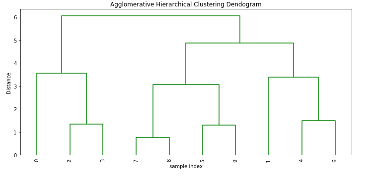
Z = linkage(custDataScaled, metric='euclidean', method='complete')
c, coph_dists = cophenet(Z , pdist(custDataScaled))
c

Output:

0.8606955190809153

plt.figure(figsize=(10, 5))
plt.title('Agglomerative Hierarchical Clustering Dendogram')
plt.xlabel('sample index')
plt.ylabel('Distance')
dendrogram(Z, leaf_rotation=90.,color_threshold=90,  leaf_font_size=10. )
plt.tight_layout()

Output:

# cophenet index is a measure of the correlation between the distance of points in feature space and distance on dendrogram
# closer it is to 1, the better is the clustering

Z = linkage(custDataScaled, metric='euclidean', method='ward')
c, coph_dists = cophenet(Z , pdist(custDataScaled))
c

Output:

0.8453818941339526

plt.figure(figsize=(10, 5))
plt.title('Agglomerative Hierarchical Clustering Dendogram')
plt.xlabel('sample index')
plt.ylabel('Distance')
dendrogram(Z, leaf_rotation=90.,color_threshold=600,  leaf_font_size=10. )
plt.tight_layout()

Output:

If you have any query or need help in any Agglomerative Hierarchical Clustering then send your request at realcode4you@gmail.com and get instant help with an affordable price.